
Reconfigurable Simple Pendulum
Reconfigurable Simple Pendulum - Theory
Learning Objectives
After completing this remote triggered experiment on simple pendulum one should be able to
- Model a given real system to an equivalent simplified model of a simple pendulum with suitable assumptions / idealizations.
- Calculate the natural frequency of the system
Introduction
A simple pendulum may be described ideally as a point mass suspended by a mass less string from some point about which it is allowed to swing back and forth in a place. A simple pendulum can be approximated by a small metal sphere which has a small radius and a large mass when compared relatively to the length and mass of the light string from which it is suspended. If a pendulum is set in motion so that is swings back and forth, its motion will be periodic. Some examples of the real life systems where principle of simple pendulum is applicable are:
- A swing on which a child can ride
- Pendulum in a grandfather's clock
- Seismometers

Pendulum on a grandfather clock is calibrated to a have a time period of 2.0s
Natural Frequency of Simple Pendulum
When the pendulum bob is displaced (small displacements) from its mean position and left, it oscillated freely about the mean position. Some of the important assumptions that are associated with the simple pendulum system are as follows:
- The mass ($m$) of the bob is the only mass in the system i.e. the string/link used to suspend the bob is mass less,
- No energy consuming element (damping) is present in the system i.e. undamped vibration,
- The complex cross section and type of material of the real system has been simplified to equate to a Cantilever beam.
The governing equation for simple pendulum in free vibration is $$ l\ddot{\theta}+g\theta= 0 $$ $$ \ddot{\theta}+ω_n^2 \theta=0 $$ $$\omega_n = \sqrt{\frac g l} $$ The time period $T$ of a simple pendulum is the time taken for one oscillation $$T=\frac{2\pi}{\omega_n} = 2\pi\sqrt{\frac l g}$$
Reconfigurable Simple Pendulum - Procedure
AIM
- Determine the damped natural frequency, logarithmic decrement and damping ratio of a given system from the free oscillation response
- Determine the effect of variation of length on above parameters
GENERAL INSTRUCTIONS
WE INSIST THAT USER READ THE INSTRUCTIONS & PROCEDURE THOROUGHLY BEFORE CARRYING OUT THE EXPERIMENT.
ONLINE and OFFLINE modes :
For the user to conduct an experiment, he/she must be connected to the SOLVE lab servers at NITK Surathkal. For this the user must be in the ONLINE mode. The user will be allowed to save the results of the online experiments and use the same for further analysis in OFFLINE mode. In case of OFFLINE mode the user is not connected to the experiment. However he/she can load a previously saved data file to get required graphs and carry out further analysis of the data. For this to happen, the user MUST have a Saved Data of the same experiment. Refer to step 6 below in procedure for downloading data.
CONTROL and VIEW modes :
In ONLINE mode, depending on availability of experiment, a user may get CONTROL or VIEW mode. In CONTROL mode the user gets to control the experiment parameters and trigger the experiment. In VIEW mode the user will not be able to control the experiment or trigger it, but will receive the data acquired during the experiment. The graph will load on screen once the data acquisition is complete. The VIEW user can chose to continue to calculations with the data received. ONLY ONE user is allowed to be in the CONTROL mode at any instant.
Allowed Actions during Remote Trigger :
While doing the experiment, i.e. when user is in Remote Trigger window, right click is permitted only in the graph area where the context menu will give options to zoom in, zoom out, save as image etc. Also, user MUST NOT REFRESH the page while carrying out an experiment. Page refreshing leads to loss of connection with the experiment server. However, the users may move back and forth between PROCEDURE tab and REMOTE TRIGGER tab while doing calculations, if they need to refer to formula given in table below.
Note: Time remaining and Number of Trials left are shown in INDICATOR block. If time is up or the number of trials left is zero the user automatically gets disconnected from the experiment server.
FORMULA
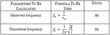
PROCEDURE:
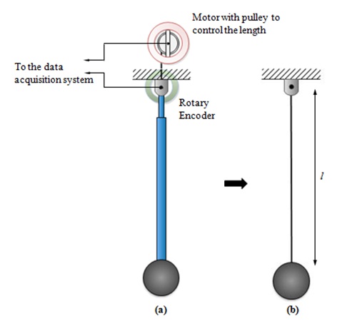
Fig 1:(a) Schematic Representation of the experimental setup; (b) Equivalent Lumped parameter system
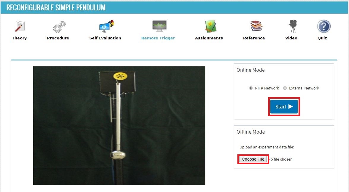
1. To conduct experiment click Start. In order to load previously saved data click on Choose file and locate the appropriate file. A pop-up dialogue box will inform you on successful loading of data. You can access the graphs and proceed to calculations once you click OK on the pop-up box. (Go to step 4 for calculations)
2. Once you are connected to the experiment server in CONTROL mode you can carry out the experiment. Depending upon the availability you will be granted CONTROL or VIEW mode. If you are granted VIEW mode you will be put in Queue and will be shown the waiting time for getting a CONTROL slot. You can either wait or you can chose to use the data acquired during ongoing session to proceed to calculations (Step 4)
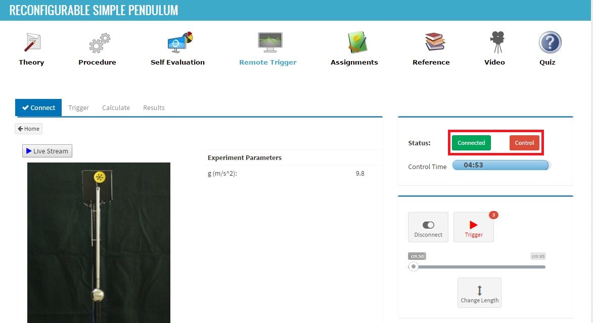
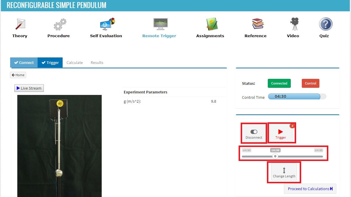
3. You can change the length of the simple pendulum. Use the slider to set the desired length and click on Change Length to actuate change of length. Click on Trigger to set the pendulum into small oscillations. The amplitude vs time data will load shortly on to your screen. Once you have received the data you may either choose to TRIGGER AGAIN or Disconnect from the experiment server. Number of trials left and the time left for you to finish the experiment are shown in Indicators block.
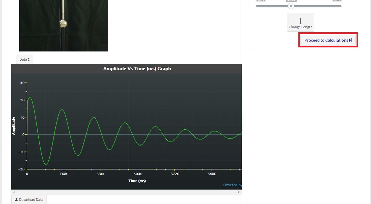
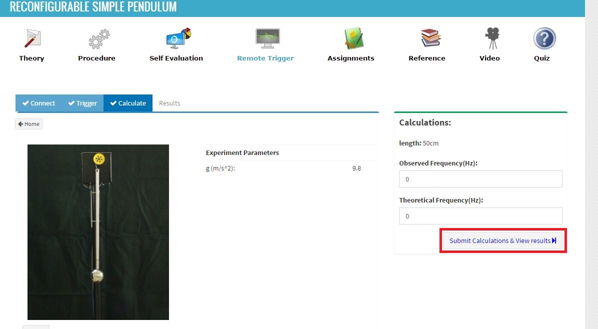
4. Click Proceed to Calculations to move to the calculations window. Known parameters are listed below the graphs. Hover over a point on the graph to find its x and y coordinates. Use available values to calculate listed parameters and enter them in appropriate fields. During calculations, the user may refer to table of formula given under the heading FORMULA above.
5. Click on Submit Calculations and View Results to submit your data. ONCE SUBMITTED ANSWERS CAN NOT BE REVERTED. A pop-up box will ask for your confirmation to submit the result. Click OK to CONTINUE. Click CANCEL if you wish to CHECK your data.
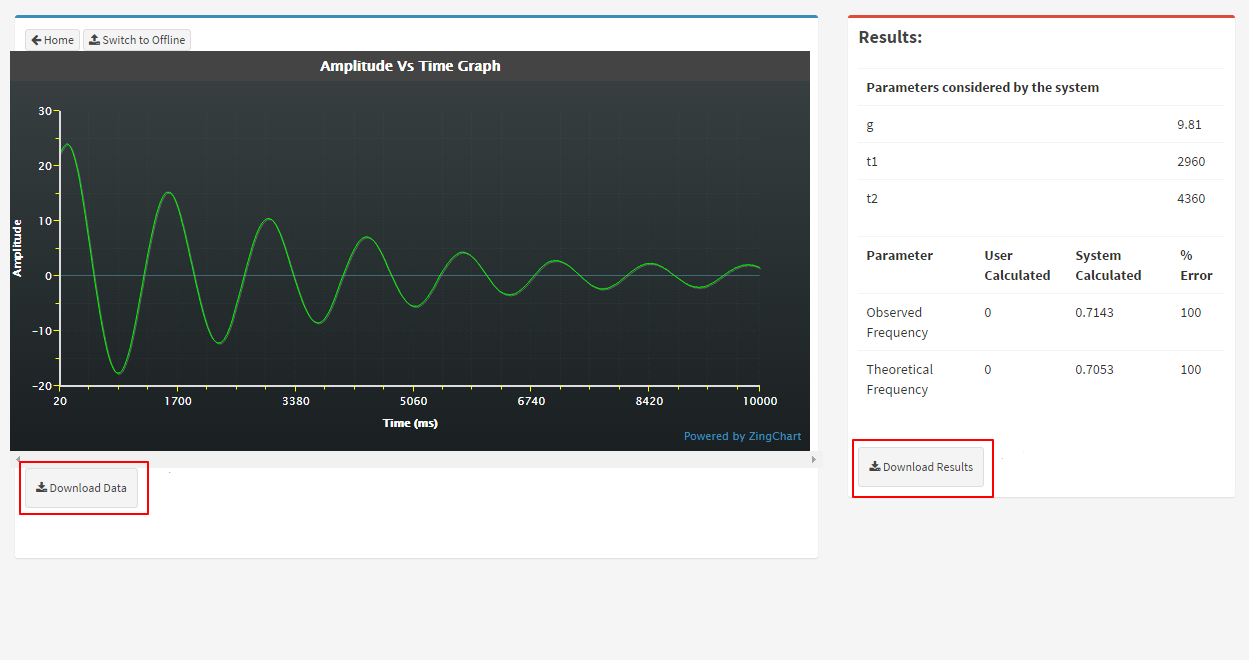
6. Click on Download Data button below the graph to download and save your data. You can use this file to load the graph and continue to calculations in the OFFLINE mode. You may also save your results (for your record) by clicking Download Results. You will receive a CSV file containing the data of your results table.
| Questions: | 4 |
| Attempts allowed: | Unlimited |
| Available: | Always |
| Pass rate: | 75 % |
| Backwards navigation: | Allowed |
Reconfigurable Simple Pendulum - Assignment
Try the following
- Plot the variation of natural frequency of simple pendulum with length of simple pendulum.
- What is ratio of natural frequency of a simple pendulum on earth and that on moon given that length of pendulum is same in both places.
- Mechanical Vibrations by "Singiresu S. Rao", Addison-Wesley Longman Incorporated, 1990
- Theory of Vibrations with Applications by "Chandramouli Padmanabhan, Marie Dillon Dahleh, William T. Thomson", Pearson Education, 2008
- Mechanical Vibration Practice and Noise Control by "V. Ramamurthi", Narosa Publishing House, 2012
- Mechanical Vibration by "Haym Benaroya and Mark L. Nagurka", CRC Press 2010
- Vibration and Acoustics by "Sujatha C", McGraw Hill Education, 2010
- Mechanical Vibrations by "G K Grover", NEM Chand & Bros, 2009
| Questions: | 4 |
| Attempts allowed: | Unlimited |
| Available: | Always |
| Pass rate: | 75 % |
| Backwards navigation: | Allowed |
Education - This is a contributing Drupal Theme
Design by WeebPal.
Design by WeebPal.