
Reconfigurable Cantilever Beam
Free Vibration of Cantilever Beam - Theory
Learning Objectives
After completing this remote triggered experiment on free vibration of a cantilever beam one should be able to:
- Model a given real system to an equivalent simplified model of a cantilever beam with suitable assumptions / idealizations.
- Calculate the logarithmic decrement, damping ratio, damping frequency and natural frequency of the system
- Find the stiffness and the critical damping of the system.
- Calculate damping coefficient of the system.
Introduction
A system is said to be a cantilever beam system if one end of the system is rigidly fixed to a support and the other end is free to move. Look at few of the real systems shown below, try to make suitable assumptions to deduce the system to a cantilever beam.
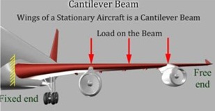
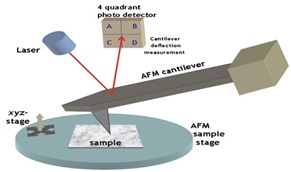
An aircraft wing as a cantilever beam An atomic force microscope probe

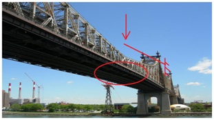
A tower crane overhang is like a cantilever beam A double overhang folding bridge
Vibration analysis of a cantilever beam system is important as it can explain and help us analyse a number of real life systems. As shown in above examples, real systems can be simplified to a cantilever beam, thereby helping us make design changes accordingly for the most efficient systems.
Natural Frequency of Cantilever Beam
When given an excitation and left to vibrate on its own, the frequency at which a cantilever beam will oscillate is its natural frequency. This condition is called Free vibration. The value of natural frequency depends only on system parameters of mass and stiffness. When a real system is approximated to a simple cantilever beam, some assumptions are made for modelling and analysis (Important assumptions for undamped system are given below):
- The mass ($m$) of the whole system is considered to be lumped at the free end of the beam
- No energy consuming element (damping) is present in the system i.e. undamped vibration
- The complex cross section and type of material of the real system has been simplified to equate to a Cantilever beam
The governing equation for such a system (spring mass system without damping under free vibration) is as below: $$ m\ddot{x}+kx= 0 $$$$ \ddot{x}+ω_n^2 x=0 $$ $$\omega_n = \sqrt{\frac k m} $$ $k$ , the stiffness of the system is a property which depends on the length ($l$), moment of inertia ($I$) and Young's Modulus ($E$) of the material of the beam and for a cantilever beam is given by: $$k=\frac{3EI}{l^3}$$
Damping in a Cantilever Beam
Although there is no visible damper (dashpot) the real system has some amount of damping contributed by the nature of the material. When a system with damping undergoes free vibration the damping property must also be considered for the modelling and analysis.
Single degree of freedom mass spring damper system under free vibration is governed by the following differential equation: $$ m\ddot{x}+c\dot{x}+kx= 0 $$ $$ \ddot{x}+2\zeta\omega_n\dot{x}+\omega_n^2 x=0 $$ $c$ is the damping present in the system and $\zeta$ is the damping factor of the system which is nothing but ratio of damping $c$ and critical damping $c_c$. Critical damping can be seen as the damping just sufficient to avoid oscillations. At critical condition $\zeta =1$. For real systems the value of $\zeta$ is less than 1. For system where $ \zeta < 1 $ the differential equation solution is a pair of complex conjugates. The displacement solution is given by $$ x(t) = e^{- \zeta \omega_n t} \left[ x_0 cos (\omega_d t) + \frac {v_0 + \zeta \omega_n x_0} {\omega_d} sin (\omega_d t) \right] $$ where $x_0$ and $v_0$ are initial displacement and velocity and $\omega_d$ is the damped natural frequency of the system. The damped natural frequency is calculated as below: $$ \omega_d = \omega_n \sqrt {1- \zeta ^2} $$
Reconfigurable Cantilever Beam - Procedure
AIM
- Determine the damped natural frequency, logarithmic decrement and damping ratio of a given system from the free vibration response
- Calculate the mass of the system actively participating in dynamics
- Determine the equivalent viscous damping present in the system
- Calculate critical damping of the system and undamped natural frequency of the system
- Determine the effect of variation of beam length on above parameters
GENERAL INSTRUCTIONS
WE INSIST THAT USER READ THE INSTRUCTIONS & PROCEDURE THOROUGHLY BEFORE CARRYING OUT THE EXPERIMENT.
ONLINE and OFFLINE modes :
For the user to conduct an experiment, he/she must be connected to the SOLVE lab servers at NITK Surathkal. For this the user must be in the ONLINE mode. The user will be allowed to save the results of the online experiments and use the same for further analysis in OFFLINE mode. In case of OFFLINE mode the user is not connected to the experiment. However he/she can load a previously saved data file to get required graphs and carry out further analysis of the data. For this to happen, the user MUST have a Saved Data of the same experiment. Refer to step 6 below in procedure for downloading data.
CONTROL and VIEW modes :
In ONLINE mode, depending on availability of experiment, a user may get CONTROL or VIEW mode. In CONTROL mode the user gets to control the experiment parameters and trigger the experiment. In VIEW mode the user will not be able to control the experiment or trigger it, but will receive the data acquired during the experiment. The graph will load on screen once the data acquisition is complete. The VIEW user can chose to continue to calculations with the data received. ONLY ONE user is allowed to be in the CONTROL mode at any instant.
Allowed Actions during Remote Trigger :
While doing the experiment, i.e. when user is in Remote Trigger window, right click is permitted only in the graph area where the context menu will give options to zoom in, zoom out, save as image etc. Also, user MUST NOT REFRESH the page while carrying out an experiment. Page refreshing leads to loss of connection with the experiment server. However, the users may move back and forth between PROCEDURE tab and REMOTE TRIGGER tab while doing calculations, if they need to refer to formula given in table below.
Note: Time remaining and Number of Trials left are shown in INDICATOR block. If time is up or the number of trials left is zero the user automatically gets disconnected from the experiment server.
FORMULA

Effective mass of cantilever beam concentrated at the free end is 0.23mbeam. So for this experiment m=msensor+0.23mbeam
PROCEDURE:
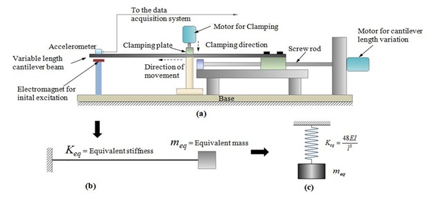
Fig 1: (a) Schematic of the experimental setup; (b) Equivalent engineering model; (c) Lumped parameter system
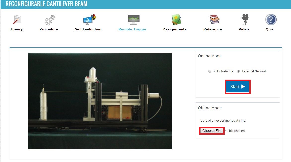
1. To conduct experiment click Start. In order to load previously saved data click on Choose file and locate the appropriate file. A pop-up dialogue box will inform you on successful loading of data. You can access the graphs and proceed to calculations once you click OK on the pop-up box. (Go to step 4 for calculations)
2. Once you are connected to the experiment server in CONTROL mode you can carry out the experiment. Depending upon the availability you will be granted CONTROL or VIEW mode. If you are granted VIEW mode you will be put in Queue and will be shown the waiting time for getting a CONTROL slot. You can either wait or you can chose to use the data acquired during ongoing session to proceed to calculations (Step 4)
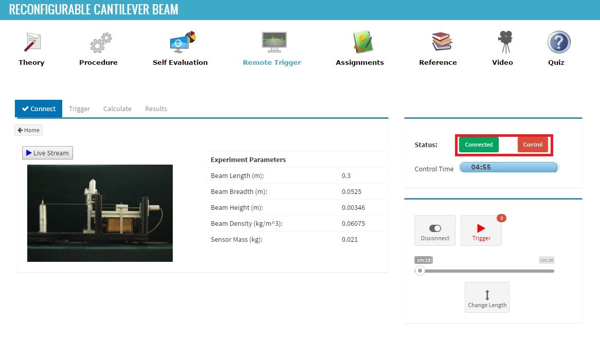
3. You can change the length of the cantilever beam. Use the slider to set the desired length and click on Change Length to actuate change of length. Click on Trigger to actuate electromagnet. The electromagnet will attract and leave the free end of the cantilever beam due to which the cantilever beam will be set into free vibration. The acceleration data from accelerometer will load shortly on to your screen. Once you have received the data you may either choose to TRIGGER AGAIN or Disconnect from the experiment server.
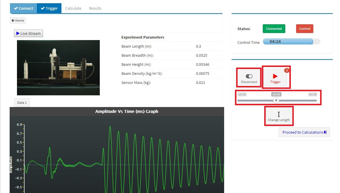
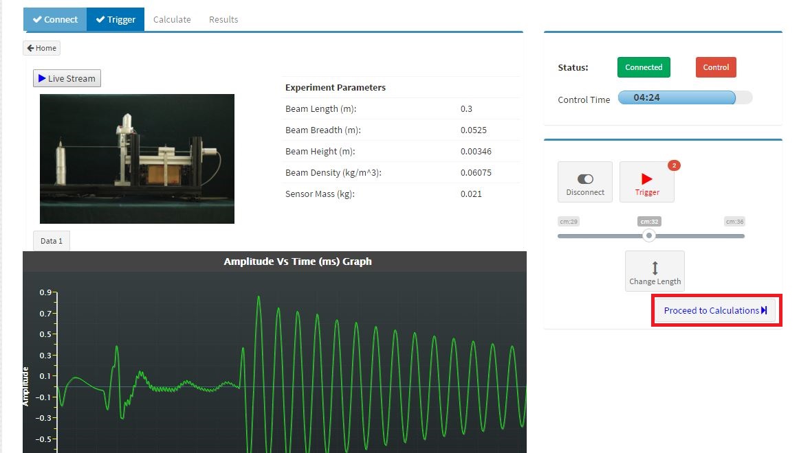
4. Click Proceed to Calculations to move to the calculations window. Known parameters are listed below the graphs. Hover over a point on the graph to find its x and y coordinates. Use available values to calculate listed parameters and enter them in appropriate fields. During calculations, the user may refer to table of formula given under the heading FORMULA above.
5. Click on Submit Calculations and View Results to submit your data. ONCE SUBMITTED ANSWERS CAN NOT BE REVERTED. A pop-up box will ask for your confirmation to submit the result. Click OK to CONTINUE. Click CANCEL if you wish to CHECK your data.

6. Click on Download Data button below the graph to download and save your data. You can use this file to load the graph and continue to calculations in the OFFLINE mode. You may also save your results (for your record) by clicking Download Results . You will receive a CSV file containing the data of your results table.

| Questions: | 4 |
| Attempts allowed: | Unlimited |
| Available: | Always |
| Pass rate: | 75 % |
| Backwards navigation: | Allowed |
Reconfigurable Cantilever Beam - Assignment
Try the following
- Plot the variation of natural frequency of cantilever beam with
- Length of Beam
- Lumped mass at free end of the beam
- What is the time taken to reduce vibration amplitude to half its initial value? How does it vary with length?
- Mechanical Vibrations by "Singiresu S. Rao", Addison-Wesley Longman Incorporated, 1990
- Theory of Vibrations with Applications by "Chandramouli Padmanabhan, Marie Dillon Dahleh, William T. Thomson", Pearson Education, 2008
- Mechanical Vibration Practice and Noise Control by "V. Ramamurthi", Narosa Publishing House, 2012
- Mechanical Vibration by "Haym Benaroya and Mark L. Nagurka", CRC Press 2010
- Vibration and Acoustics by "Sujatha C", McGraw Hill Education, 2010
- Mechanical Vibrations by "G K Grover", NEM Chand & Bros, 2009
| Questions: | 4 |
| Attempts allowed: | Unlimited |
| Available: | Always |
| Pass rate: | 75 % |
| Backwards navigation: | Allowed |
Education - This is a contributing Drupal Theme
Design by WeebPal.
Design by WeebPal.